Two-point flux-approximation (TPFA) for Darcy flow

Last updated on Oct 21, 2022

Results from this method

Projects description

Purpose: This is my notes for using Matplotlib to make animation, it’s very convenient during your simulation.

1.1 Functions

1.1.1 Basic Functions

Continuity function

$\begin{matrix} (1.1) & \frac{\partial (ϕ ρ)}{\partial t} + ▽ \cdot (ρ v) = q \end{matrix}$ where $ϕ$ is the porosity, $ρ$ is the density, $v$ is the flow velocities and $q$ is the source term which models sources and sinks ( outflow and inflow per volume at designated well locations).

Darcy Law

$\begin{matrix} (1.2) & v = - \frac{K}{μ} (▽ p + ρ g ▽ z) \end{matrix}$

1.1.2 Instance: for water

Simplicity: $ϕ$ and $ρ$ is constant in time. The first term(temporal derivative term) in (1.1) equals to 0.
Calculating the divergence for $v$ : $▽ \cdot v_{w}$
From eq. (1.1): $▽ \cdot v_{w} = \frac{q_{w}}{ρ_{w}}$ ,
and from eq. (1.2): $▽ \cdot v_{w} = ▽ \cdot [- \frac{K}{μ_{w}} (▽ p_{w} + ρ_{w} G)]$ .
So, we can get equation (1.3), where the lower label $_{w}$ means properties for water.

$\begin{matrix} (1.3) & ▽ \cdot v_{w} = \frac{q_{w}}{ρ_{w}} = ▽ \cdot [- \frac{K}{μ_{w}} (▽ p_{w} + ρ_{w} G)] \end{matrix}$

Bundary condition on the reservoir boundary $\partial Ω$ , where the $n$ is the normal vector pointing out of the boundary $\partial Ω$ $\begin{matrix} (1.4) & v_{w} \cdot n = 0 \end{matrix}$
Understanding Let’s take a look at Eq. (1.3), on the left side (the first equality), $v_{w}$ is unknown, and on the right side, the $p_{w}$ is unknown, only the $q_{w}$ and $ρ_{w}$ is known. So ,the $v_{w}$ and $p_{w}$ are the parameters need to be solved with $q_{w}$ and $ρ_{w}$ in TPFA scheme.

1.2 TPFA(Two-point flux-approximation)

TPFA scheme, is a cell-centred finite-volume method, which is also one of the simplest discretization techniques for elliptic equations.

1.2.1 Functions of the $v_{w}$

$Ω_{i}$ stands for a grid cell in $Ω$ , then consider the following integral over in $Ω_{i}$

$\begin{matrix} (1.5) & \int_{Ω_{i}} (\frac{q_{w}}{ρ_{w}} - ▽ \cdot v_{w}) d x = 0 \end{matrix}$

Obviously, it’s coming from the left two term of Eq.(1.5).

Assuming that $v_{w}$ is smooth, then apply the divergence theorem: $\int_{Ω} ▽ \cdot a d Ω = \int_{\partial Ω} n \cdot a d \partial Ω$

$\begin{matrix} (1.6) & \int_{\partial Ω_{i}} v_{w} \cdot n d \partial Ω_{i} = \int_{Ω_{i}} (\frac{q_{w}}{ρ_{w}}) d Ω_{i} \end{matrix}$

Attention: $Ω_{i}$ is the volume of one finite volume(or a cell), $\partial Ω_{i}$ stands for the surface of one finite volume(or a cell), and $γ_{i j} = \partial Ω_{i} \cap \partial Ω_{j}$ is the interfaces of two neighbor cells.

Summary Obviously, the left term in Eq.(1.6) is unknown (the $v_{w}$ ), and the right term is already known ( $q_{w}$ is coming from the initial condition and $ρ_{w}$ is constant in this problem). So, we can get $v_{w}$ in each cell by calculating Eq.(1.6). But in current problem, the solving of $p_{w}$ is much harder, so, we use TPFA to solve the $p_{w}$ first,then solve the $v_{w}$ by $p_{w}$ according to Eq. (1.2).

1.2.2 Functions the $p$

Making $u_{w} = p_{w} + ρ_{w} g z$ and $λ = \frac{K}{μ_{w}}$
Reformulate Eq.(1.3) to get the proper equation like the Eq.(1,6), which is the standard TPFA FVM scheme. $\begin{matrix} (1.7) & - ▽ \cdot λ ▽ u_{w} = \frac{q_{w}}{ρ_{w}} \end{matrix}$
Integrate over the finite volume $\begin{matrix} (1.8) & \int_{Ω} - ▽ \cdot λ ▽ u_{w} d Ω = \int_{Ω} \frac{q_{w}}{ρ_{w}} d Ω \end{matrix}$
Apply the divergence theorem $\begin{matrix} (1.9) & \int_{Ω} - ▽ \cdot λ ▽ u_{w} d Ω = \int_{\partial Ω} (λ ▽ u_{w}) d Ω \end{matrix}$
As ,the u_w only changes between cells, the $\partial Ω$ changes into $γ_{i j}$ , which is the interface of two neighboring cells. $$\int {\Omega}-\bigtriangledown \cdot \lambda \bigtriangledown u_w d\Omega=\int {\gamma{ij}}(\lambda \bigtriangledown u_w)d\gamma{ij} \tag{1.10}$$
So, finally, we can get:

$$\int {\Omega}\frac{q_w}{\rho_w}d\Omega=\int {\gamma{ij}}(\lambda \bigtriangledown u_w)d\gamma{ij} \tag{1.11}$$

1.2.3 Discretization

Let’s discretization with Eq. (1.11) and adding a flux term $v_{i j}$ . The reason why we have to discretize the parameter is that in FVM method, we assume all the parameters are cell-wise constant, we have to discretize them to get the proper value on the interface $λ_{i j}$

Discretization of $u$ : As this is a regular hexahedral grid with gridlines aligned with the principal coordinate axes, in the x-coordinate direction, $n_{i j} = (1, 0, 0)^{T}$ , and the $△ x_{j}$ and the $△ x_{i}$ denote the respective cell dimensions in the x-coordinate direction. So the $▽ u_{w}$ on $γ_{i j}$ can be discretized into:
$\begin{matrix} (1.12) & ▽ u_{w} = δ u_{i j} = \frac{(u_{j} - u_{i})}{\frac{△ x_{j} + △ x_{i}}{2}} \end{matrix}$
Discretization of $λ$ : The permeability, in the TPFA method this is done by taking a distance-weighted harmonic average of the respective directional cell permeability.(即对相邻网格进行网格步长的加权平均)
$\begin{matrix} (1.13) & λ_{i j} = (△ x_{i} + △ x_{j}) (\frac{△ x_{i}}{λ_{i, i j}} + \frac{△ x_{j}}{λ_{j, i j}})^{- 1} \end{matrix}$
Discretization of Eq. (1.11):

$$v_{ij}=-|\gamma {ij}|\lambda{ij}\delta u_{ij}=2|\gamma _{ij}|(\frac{\bigtriangleup x_i}{\lambda _{i,ij}}+\frac{\bigtriangleup x_j}{\lambda _{j,ij}})^{-1}(u_i-u_j) \tag{1.14}$$

1.2.4 Solve the $u$

Simplize Eq.(1.14) Terms that do not involve the cell potentials $u_{i}$ (unknown term) are usually gathered into an interface transmissibility $t_{i} j$ (known term): $t_{i j} = 2 | γ_{i j} | (\frac{△ x_{i}}{λ_{i, i j}} + \frac{△ x_{j}}{λ_{j, i j}})^{- 1}$ , so we can get:
$\begin{matrix} (1.15) & \sum_{j} t_{i j} (u_{i} - u_{j}) = \int_{Ω} \frac{q_{w}}{ρ_{w}} d Ω \end{matrix}$
Solve the function According to Eq. (1.15), only $u_{i}$ and $u_{j}$ are unknown, so, we can solve this function to get all $u_{i}$ .

1.2.5 Solve the $v$

Function According to Eq.(1.2) and with some new parameters we defined during the process. $\begin{matrix} (1.16) & v = - λ ▽ u_{w} \end{matrix}$
Discretization According to Eq. (1.12), we can get: $\begin{matrix} (1.17) & v = - λ \frac{(u_{j} - u_{i})}{\frac{△ x_{j} + △ x_{i}}{2}} \end{matrix}$
Solve the function As the $u_{i}$ and $u_{j}$ are solved in former process, the $v$ can be solved. But notice that $u_{i}$ (u[0:-1] in code) is ahead of $u_{j}$ (u[1:] in code).

1.3 Code

1.3.1 Numpy version

# -*- coding: utf-8 -*-
"""
Created on Sun Aug  7 11:00:33 2022

@author: Howw
"""
import numpy as np
import matplotlib.pyplot as plt
import scipy.ndimage
from scipy.sparse import spdiags
from struct_tools import DotDict
np.random.seed(42)

# TPFA(two-point flux-approrimation) finite-volume discretisation
def TPFA(Nx,Ny, K, q):

    # Compute transmissibilities
    hx,hy=1/Nx,1/Ny
    L = K**(-1)
    ''' this is the t_ij in function(see notes), 
    as cell in current problem is same-wise (in the same direction, so \delta xi= \delta xj)
    and for 2-D problem, the area of cell equals to dx or dy.
    '''
    TX = np.zeros((Nx+1, Ny))
    TY = np.zeros((Nx,   Ny+1))
    TX[1:-1, :] = 2*hy/hx/(L[0, :-1, :] + L[0, 1:, :])
    TY[:, 1:-1] = 2*hx/hy/(L[1, :, :-1] + L[1, :, 1:])

    # Assemble TPFA discretization matrix, Ravel is better than reshape(N,1)
    x1 = TX[:-1, :].ravel()
    x2 = TX[1:, :] .ravel()
    y1 = TY[:, :-1].ravel()
    y2 = TY[:, 1:] .ravel()

    ## Setup linear system(confused?)
    DiagVecs = [-x2,   -y2, y1+y2+x1+x2, -y1,  -x1]
    DiagIndx = [-Ny,  -1,      0,        1,    Ny]
    ## Coerce system to be SPD
    DiagVecs[2][0] += np.sum(K[:, 0, 0])
    A = spdiags(DiagVecs, DiagIndx,N,N).toarray()

    ## Solve to get all u
    u = np.linalg.solve(A, q)

    # Get fluxes, V, of each cell
    P = u.reshape(Nx,Ny)
    # use DotDict from sturct_tool to make V become 2-D with matrix
    V = DotDict(
        x = np.zeros((Nx+1, Ny)),
        y = np.zeros((Nx, Ny+1)),  
        )
    V.x[1:-1, :] = (P[:-1, :] - P[1:, :]) * TX[1:-1, :]
    V.y[:, 1:-1] = (P[:, :-1] - P[:, 1:]) * TY[:, 1:-1]
    
    # Get velocity of each cell
    v=DotDict(
        x = np.zeros((Nx+1, Ny)),
        y = np.zeros((Nx, Ny+1)), 
        )
    v.x[1:-1,:]=-TX[1:-1,:]*(P[1:,:]-P[:-1,:])/(hx)
    v.y[:,1:-1]=-TY[:,1:-1]*(P[:,1:]-P[:,:-1])/(hy)
    
    return P, V, v

Nx,Ny=32,32
N=Nx*Ny
# K=np.ones((3,8,8))
# K=np.exp(5* ((np.random.rand(3, Nx, Ny))))
K=np.exp(5* scipy.ndimage.uniform_filter((np.random.rand(3, Nx, Ny)),5))
q=np.zeros(N)
q[0]=1
q[-1]=-1

#p is the pressure, V is the flux, v is the velocity
P,V, v=TPFA(Nx,Ny,K,q)

#draw the results
levels=np.linspace(P.min(),P.max(),20)
Grid_X=np.linspace(0,1,Nx)
Grid_Y=np.linspace(0,1,Ny)

plt.contourf(Grid_X,Grid_Y,P,levels=levels)
plt.savefig("./figures/p.png",dpi=100,bbox_inches="tight")
plt.contourf(Grid_X,Grid_Y,v.x[:-1,:])
plt.savefig("./figures/vx.png",dpi=100,bbox_inches="tight")
plt.contourf(Grid_X,Grid_Y,v.y[:,:-1])
plt.savefig("./figures/vy.png",dpi=100,bbox_inches="tight")

1.3.2 Torch version

# -*- coding: utf-8 -*-
"""
Created on Sun Aug  7 11:00:33 2022

@author: Howw
"""
import numpy as np
import torch
import matplotlib.pyplot as plt
import scipy.ndimage
from struct_tools import DotDict
import time
random_seed=42

#this function is based on torch, acted like scipy.sparse.sodiags
#data should be 1-D,and diags should be an int
def torch_spdiags(data,diags):
    data_out=torch.zeros(data.shape[0],data.shape[0])
    if diags==0:
        data_out=data_out+torch.diagflat(data,0)
    if diags>0:
        data_out=data_out+torch.diagflat(data[diags:],diags)
    if diags<0:
        data_out=data_out+torch.diagflat(data[:diags],diags)
    return data_out

# TPFA(two-point flux-approrimation) finite-volume discretisation
def TPFA(Nx,Ny, K, q):

    # Compute transmissibilities by harmonic averaging.
    hx,hy=1/Nx,1/Ny
    L = K**(-1)
    TX = torch.zeros((Nx+1, Ny))
    TY = torch.zeros((Nx,   Ny+1))
    
    TX[1:-1, :] = 2*hy/hx/(L[0, :-1, :] + L[0, 1:, :])
    TY[:, 1:-1] = 2*hx/hy/(L[1, :, :-1] + L[1, :, 1:])

    # Assemble TPFA discretization matrix, Ravel is better than reshape(N,1)
    x1 = TX[:-1, :].ravel()
    x2 = TX[1:, :] .ravel()
    y1 = TY[:, :-1].ravel()
    y2 = TY[:, 1:] .ravel()

    ## Setup linear system(confused?)
    ## Coerce system to be SPD (ref article, page 13).

    ## Version 1: failed in always using torch
    ##Attention: as I failed in find spdiags in Torch, Here the SPD is still using scipy and numpy
    # DiagVecs = [-x2.numpy(),   -y2.numpy(), (y1+y2+x1+x2).numpy(), -y1.numpy(),  -x1.numpy()]
    # DiagIndx = [-Ny,  -1,      0,        1,    Ny]
    # A_temp=spdiags(DiagVecs, DiagIndx,N,N).toarray()
    # A = torch.from_numpy(A_temp)
    
    ## Version 2:successfully using torch all the time by self-defined function
    DiagVecs =[-x2,   -y2, (y1+y2+x1+x2), -y1,  -x1]
    DiagVecs[2][0] += torch.sum(K[:, 0, 0])
    A=torch_spdiags(DiagVecs[0],-Ny)+torch_spdiags(DiagVecs[1],-1)+\
        torch_spdiags(DiagVecs[2],0)+torch_spdiags(DiagVecs[3],1)+torch_spdiags(DiagVecs[4],Ny)

    ## Solve
    u = torch.linalg.solve(A, q)

    # Extract fluxes
    P = u.reshape(Nx,Ny)
    # use DotDict from sturct_tool to make V become 2-D with matrix
    V = DotDict(
        x = torch.zeros((Nx+1, Ny)),
        y = torch.zeros((Nx, Ny+1)),  # noqa
        )
    V.x[1:-1, :] = (P[:-1, :] - P[1:, :]) * TX[1:-1, :]
    V.y[:, 1:-1] = (P[:, :-1] - P[:, 1:]) * TY[:, 1:-1]
    
    # Get velocity of each cell
    v=DotDict(
        x = torch.zeros((Nx+1, Ny)),
        y = torch.zeros((Nx, Ny+1)), 
        )
    v.x[1:-1,:]=-TX[1:-1,:]*(P[1:,:]-P[:-1,:])/(hx)
    v.y[:,1:-1]=-TY[:,1:-1]*(P[:,1:]-P[:,:-1])/(hy)
    return P, V,v

#loss function based on Eq. 1.17
def loss_TPFA(P,v,Nx,Ny,K):
    hx,hy=1/Nx,1/Ny
    L = K**(-1)
    Lamada_x = torch.zeros((Nx+1, Ny))
    Lamada_y = torch.zeros((Nx,   Ny+1))
    Lamada_x[1:-1, :] = 2*hy/hx/(L[0, :-1, :] + L[0, 1:, :])
    Lamada_y[:, 1:-1] = 2*hx/hy/(L[1, :, :-1] + L[1, :, 1:])
    loss_x=v.x[1:-1,:]+Lamada_x[1:-1,:]*(P[1:,:]-P[:-1,:])/hx
    loss_y=v.y[:,1:-1]+Lamada_y[:,1:-1]*(P[:,1:]-P[:,:-1])/hy
    return loss_x,loss_y
    

#Initializing 
Nx,Ny=64,64
N=Nx*Ny
# K=np.ones((3,8,8))
# K=np.exp(5* ((np.random.rand(3, Nx, Ny))))
K=np.exp(5* scipy.ndimage.uniform_filter((np.random.rand(3, Nx, Ny)),5))
K=torch.from_numpy(K)
q=torch.zeros(N)
q[0]=1
q[-1]=-1
start = time.perf_counter()
P,V,v=TPFA(Nx,Ny,K,q)
end = time.perf_counter()
print("Time:",end-start)
loss_x,loss_y=loss_TPFA(P,v,Nx,Ny,K)


#Draw the distribution of pressure
levels=np.linspace(P.min(),P.max(),20)
Grid_X=np.linspace(0,1,Nx)
Grid_Y=np.linspace(0,1,Ny)
# plt.contourf(Grid_X,Grid_Y,P,levels=levels)
# plt.contourf(Grid_X,Grid_Y,P,levels=levels)
# plt.savefig("./figures/p.png",dpi=100,bbox_inches="tight")
# plt.contourf(Grid_X,Grid_Y,v.x[:-1,:])
# plt.savefig("./figures/vx.png",dpi=100,bbox_inches="tight")
# plt.contourf(Grid_X,Grid_Y,v.y[:,:-1])
# plt.savefig("./figures/vy.png",dpi=100,bbox_inches="tight")

1.4 Loss function

1.4.1 Description

As this work is used for generating data for Operator training, it’s better to difine a loss function in advance, which can help the training process as combined with MSE.

1.4.2 Definition

In this work, only one function ban be uesd as loss function as there is no useful initial condition of $v$ , $v$ is calculated by Eq. (1.17), and as it’s coming form difference of $u$ , the value on the boundary can’t be calculated, so only $v . x [N x - 1, N y]$ and $v . y [N x, N y - 1]$ can be calculated.

Let’s take a look at code for calculating $v$

v=DotDict(
    x = np.zeros((Nx+1, Ny)),
    y = np.zeros((Nx, Ny+1)), 
        )
    v.x[1:-1,:]=-TX[1:-1,:]*(P[1:,:]-P[:-1,:])/(hx)
    v.y[:,1:-1]=-TY[:,1:-1]*(P[:,1:]-P[:,:-1])/(hy)

And showing the process with sketching:

So, only function (1.17) can be uesd as loss function, as other functions, like Eq. 1.1, containing q(Nx*Ny), which can’t be used with $v$ .

1.4.3 Code

#loss function based on Eq. 1.17
def loss_TPFA(P,v,Nx,Ny,K):
    hx,hy=1/Nx,1/Ny
    L = K**(-1)
    Lamada_x = np.zeros((Nx+1, Ny))
    Lamada_y = np.zeros((Nx,   Ny+1))
    Lamada_x[1:-1, :] = 2*hy/hx/(L[0, :-1, :] + L[0, 1:, :])
    Lamada_y[:, 1:-1] = 2*hx/hy/(L[1, :, :-1] + L[1, :, 1:])
    loss_x=v.x[1:-1,:]+Lamada_x[1:-1,:]*(P[1:,:]-P[:-1,:])/hx
    loss_y=v.y[:,1:-1]+Lamada_y[:,1:-1]*(P[:,1:]-P[:,:-1])/hy
    return loss_x,loss_y

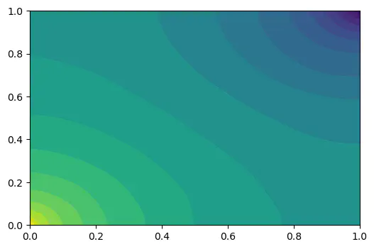
1.5 Results

1.5.1 The distribution of pressure

1.5.1 The distribution of velocity

v_x

v_y

Reference

G. Hasle, K.-A. Lie, E. Quak, and Selskapet for industriell og teknisk forskning ved Norges tekniske høgskole, Eds., Geometric modelling, numerical simulation, and optimization: applied mathematics at SINTEF. Berlin ; New York : [Oslo]: Springer ; SINTEF, 2007.

Simulation

Two-point flux-approximation (TPFA) for Darcy flow

Projects description

1.1 Functions

1.1.1 Basic Functions

1.1.2 Instance: for water

1.2 TPFA(Two-point flux-approximation)

1.2.1 Functions of the $v_{w}$

1.2.2 Functions the $p$

1.2.3 Discretization

1.2.4 Solve the $u$

1.2.5 Solve the $v$

1.3 Code

1.3.1 Numpy version

1.3.2 Torch version

1.4 Loss function

1.4.1 Description

1.4.2 Definition

1.4.3 Code

1.5 Results

1.5.1 The distribution of pressure

1.5.1 The distribution of velocity

Reference

Hao Wei

Computation, Modelling, and Reconstruction

Two-point flux-approximation (TPFA) for Darcy flow

Projects description

1.1 Functions

1.1.1 Basic Functions

1.1.2 Instance: for water

1.2 TPFA(Two-point flux-approximation)

1.2.1 Functions of the vw

1.2.2 Functions the p

1.2.3 Discretization

1.2.4 Solve the u

1.2.5 Solve the v

1.3 Code

1.3.1 Numpy version

1.3.2 Torch version

1.4 Loss function

1.4.1 Description

1.4.2 Definition

1.4.3 Code

1.5 Results

1.5.1 The distribution of pressure

1.5.1 The distribution of velocity

Reference

Hao Wei

Computation, Modelling, and Reconstruction

1.2.1 Functions of the $v_{w}$

1.2.2 Functions the $p$

1.2.4 Solve the $u$

1.2.5 Solve the $v$