FDM solver for incompressible flow

Last updated on Oct 22, 2022

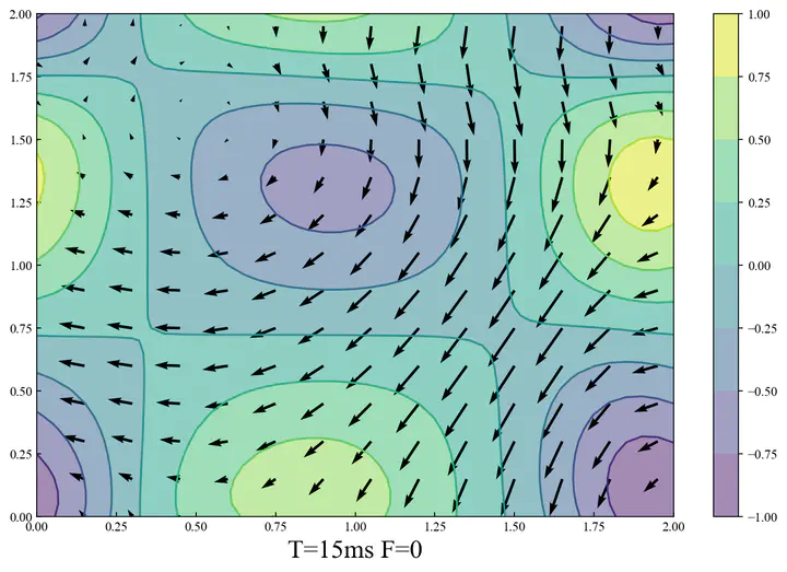Photo of the distribution of velocity

Description

In this note, I will introduce a channel flow case, solved by Finite Difference Method.

The initial velocity is generated by Taylor_green vortex, with a force in x-axis towards the right, making the fluid moving to the right direction.

The boundary conditions are: periodic for the inlet and outlet, no-slip for the top and bottom.

There are two different methods for solving pressure, one is the simple algorithm from Anderson’s book, the other is the possion equations.

Equations

In this case, there is a source term (F) in the $u$ -momentum equation. Here are our modified Navier–Stokes equations:

This will solve the Navier–Stokes equations in two dimensions, with boundary conditions.

The momentum equation in vector form for a velocity field $\vec{v}$ is:

$\frac{\partial \vec{v}}{\partial t} + (\vec{v} \cdot \nabla) \vec{v} = - \frac{1}{ρ} \nabla p + ν \nabla^{2} \vec{v} + F_{x}$

The continuity equation in vector form for a velocity field $\vec{v}$ is:

$\nabla \cdot \vec{v} = 0$

Continuity：

$\frac{\partial u}{\partial x} + \frac{\partial v}{\partial y} = 0$

Momentum:

$\frac{\partial u}{\partial t} + u \frac{\partial u}{\partial x} + v \frac{\partial u}{\partial y} = - \frac{1}{ρ} \frac{\partial p}{\partial x} + ν (\frac{\partial^{2} u}{\partial x^{2}} + \frac{\partial^{2} u}{\partial y^{2}}) + F_{x}$

$\frac{\partial v}{\partial t} + u \frac{\partial v}{\partial x} + v \frac{\partial v}{\partial y} = - \frac{1}{ρ} \frac{\partial p}{\partial y} + ν (\frac{\partial^{2} v}{\partial x^{2}} + \frac{\partial^{2} v}{\partial y^{2}})$

Discretization

First, let’s discretize the momentum equation, as follows:

The momentum equation is the key to update the velocity with pressure, while the continuity equation is used to midify the pressure.

$u$ -momentum equation: $\begin{aligned} \frac{u_{i, j}^{n + 1} - u_{i, j}^{n}}{Δ t} + u_{i, j}^{n} \frac{u_{i, j}^{n} - u_{i - 1, j}^{n}}{Δ x} + v_{i, j}^{n} \frac{u_{i, j}^{n} - u_{i, j - 1}^{n}}{Δ y} = & - \frac{1}{ρ} \frac{p_{i + 1, j}^{n} - p_{i - 1, j}^{n}}{2 Δ x} + ν (\frac{u_{i + 1, j}^{n} - 2 u_{i, j}^{n} + u_{i - 1, j}^{n}}{Δ x^{2}} + \frac{u_{i, j + 1}^{n} - 2 u_{i, j}^{n} + u_{i, j - 1}^{n}}{Δ y^{2}}) + F_{x} \end{aligned}$ $v$ -momentum equation: $\begin{aligned} \frac{v_{i, j}^{n + 1} - v_{i, j}^{n}}{Δ t} + u_{i, j}^{n} \frac{v_{i, j}^{n} - v_{i - 1, j}^{n}}{Δ x} + v_{i, j}^{n} \frac{v_{i, j}^{n} - v_{i, j - 1}^{n}}{Δ y} = & - \frac{1}{ρ} \frac{p_{i, j + 1}^{n} - p_{i, j - 1}^{n}}{2 Δ y} + ν (\frac{v_{i + 1, j}^{n} - 2 v_{i, j}^{n} + v_{i - 1, j}^{n}}{Δ x^{2}} + \frac{v_{i, j + 1}^{n} - 2 v_{i, j}^{n} + v_{i, j - 1}^{n}}{Δ y^{2}}) \end{aligned}$

Rearrange

Rearrange the equations in the way that easy for the iterations during calculation

$u_{i, j}^{n + 1} = u_{i, j}^{n} - \frac{Δ t}{ρ 2 Δ x} (p_{i + 1, j}^{n} - p_{i - 1, j}^{n}) + (A + F_{x}) Δ t$

$\begin{array}{r} A = [- \frac{u_{i, j}^{n}}{Δ x} (u_{i, j}^{n} - u_{i - 1, j}^{n}) - \frac{v_{i, j}^{n}}{Δ y} (u_{i, j}^{n} - u_{i, j - 1}^{n}) + \frac{ν}{Δ x^{2}} (u_{i + 1, j}^{n} - 2 u_{i, j}^{n} + u_{i - 1, j}^{n}) + \frac{ν}{Δ y^{2}} (u_{i, j + 1}^{n} - 2 u_{i, j}^{n} + u_{i, j - 1}^{n})] \end{array}$

$v_{i, j}^{n + 1} = v_{i, j}^{n} - - \frac{Δ t}{ρ 2 Δ y} (p_{i, j + 1}^{n} - p_{i, j - 1}^{n}) + B Δ t$

$B = [- \frac{u_{i, j}^{n}}{Δ x} (v_{i, j}^{n} - v_{i - 1, j}^{n}) - \frac{v_{i, j}^{n}}{Δ y} (v_{i, j}^{n} - v_{i, j - 1}^{n})) + \frac{ν}{Δ x^{2}} (v_{i + 1, j}^{n} - 2 v_{i, j}^{n} + v_{i - 1, j}^{n}) + \frac{ν}{Δ y^{2}} (v_{i, j + 1}^{n} - 2 v_{i, j}^{n} + v_{i, j - 1}^{n})]$

Pressure modification Method 1: Simple algorithm

$$p^{n+1}{i,j}=p^{n}{i,j}+\alpha_n p’_{i,j}$$

In which, $α_{n}$ is the relaxation factor, herein, we set as 0.1

$$ap’{i,j}+bp’{i+1,j}+bp’{i-1,j}+cp’{i,j+1}cp’_{i,j-1}+d=0$$

$b = - \frac{1}{ρ} \frac{Δ t}{(Δ x)^{2}}$

$c = - \frac{1}{ρ} \frac{Δ t}{(Δ y)^{2}}$

$a = \frac{2}{ρ} [\frac{Δ t}{(Δ x)^{2}} + \frac{Δ t}{(Δ y)^{2}}] = - 2 (b + c)$

$d = \frac{1}{Δ x} [u_{i + 1, j}^{n} - u_{i - 1, j}^{n}] + \frac{1}{Δ y} [v_{i, j + 1}^{n} - v_{i, j - 1}^{n}]$

Pressure modification Method 2: Passion Equation

$\frac{\partial^{2} p}{\partial x^{2}} + \frac{\partial^{2} p}{\partial y^{2}} = - ρ (\frac{\partial u}{\partial x} \frac{\partial u}{\partial x} + 2 \frac{\partial u}{\partial y} \frac{\partial v}{\partial x} + \frac{\partial v}{\partial y} \frac{\partial v}{\partial y})$

Discretization

$\begin{aligned} \frac{p_{i + 1, j}^{n} - 2 p_{i, j}^{n} + p_{i - 1, j}^{n}}{Δ x^{2}} + \frac{p_{i, j + 1}^{n} - 2 p_{i, j}^{n} + p_{i, j - 1}^{n}}{Δ y^{2}} = & ρ [\frac{1}{Δ t} (\frac{u_{i + 1, j} - u_{i - 1, j}}{2 Δ x} + \frac{v_{i, j + 1} - v_{i, j - 1}}{2 Δ y}) - \frac{u_{i + 1, j} - u_{i - 1, j}}{2 Δ x} \frac{u_{i + 1, j} - u_{i - 1, j}}{2 Δ x} - 2 \frac{u_{i, j + 1} - u_{i, j - 1}}{2 Δ y} \frac{v_{i + 1, j} - v_{i - 1, j}}{2 Δ x} - \frac{v_{i, j + 1} - v_{i, j - 1}}{2 Δ y} \frac{v_{i, j + 1} - v_{i, j - 1}}{2 Δ y}] \end{aligned}$

Rearrange

$\begin{aligned} p_{i, j}^{n} = & \frac{(p_{i + 1, j}^{n} + p_{i - 1, j}^{n}) Δ y^{2} + (p_{i, j + 1}^{n} + p_{i, j - 1}^{n}) Δ x^{2}}{2 (Δ x^{2} + Δ y^{2})} & - \frac{ρ Δ x^{2} Δ y^{2}}{2 (Δ x^{2} + Δ y^{2})} & \times [\frac{1}{Δ t} (\frac{u_{i + 1, j} - u_{i - 1, j}}{2 Δ x} + \frac{v_{i, j + 1} - v_{i, j - 1}}{2 Δ y}) - \frac{u_{i + 1, j} - u_{i - 1, j}}{2 Δ x} \frac{u_{i + 1, j} - u_{i - 1, j}}{2 Δ x} - 2 \frac{u_{i, j + 1} - u_{i, j - 1}}{2 Δ y} \frac{v_{i + 1, j} - v_{i - 1, j}}{2 Δ x} - \frac{v_{i, j + 1} - v_{i, j - 1}}{2 Δ y} \frac{v_{i, j + 1} - v_{i, j - 1}}{2 Δ y}] \end{aligned}$

Assuming the b equals to: $ρ [\frac{1}{Δ t} (\frac{u_{i + 1, j} - u_{i - 1, j}}{2 Δ x} + \frac{v_{i, j + 1} - v_{i, j - 1}}{2 Δ y}) - \frac{u_{i + 1, j} - u_{i - 1, j}}{2 Δ x} \frac{u_{i + 1, j} - u_{i - 1, j}}{2 Δ x} - 2 \frac{u_{i, j + 1} - u_{i, j - 1}}{2 Δ y} \frac{v_{i + 1, j} - v_{i - 1, j}}{2 Δ x} - \frac{v_{i, j + 1} - v_{i, j - 1}}{2 Δ y} \frac{v_{i, j + 1} - v_{i, j - 1}}{2 Δ y}]$

Then $\begin{aligned} p_{i, j}^{n} = & \frac{(p_{i + 1, j}^{n} + p_{i - 1, j}^{n}) Δ y^{2} + (p_{i, j + 1}^{n} + p_{i, j - 1}^{n}) Δ x^{2}}{2 (Δ x^{2} + Δ y^{2})} - \frac{b Δ x^{2} Δ y^{2}}{2 (Δ x^{2} + Δ y^{2})} \end{aligned}$

Initial and boundary condition

The initial condition is $u, v, p = 0$ everywhere.

boundary conditions:

$u, v, p$ are periodic on $x = 0, 2$

$u, v = 0$ at $y = 0, 2$

$\frac{\partial p}{\partial y} = 0$ at $y = 0, 2$

$F = 1$ everywhere.

Code

Let’s Coding!

import numpy as np
from matplotlib import pyplot as plt
from matplotlib import cm

def cal_A(dx,dy,nu,u_in,v_in):
    u=u_in.copy().astype(np.float32)
    v=v_in.copy().astype(np.float32)
    A=np.zeros_like(u).astype(np.float32)
    #interior
    A[1:-1,1:-1]=-u[1:-1,1:-1]/dx*(u[1:-1,1:-1]-u[1:-1,0:-2])\
                 -v[1:-1,1:-1]/dy*(u[1:-1,1:-1]-u[0:-2,1:-1])\
                 +nu/((dx)**2)*(u[1:-1,2:]-2*u[1:-1,1:-1]+u[1:-1,0:-2])\
                 +nu/((dy)**2)*(u[2:,1:-1]-2*u[1:-1,1:-1]+u[0:-2,1:-1])

    #periodic boundary x=0
    A[1:-1,0]=-u[1:-1,0]/dx*(u[1:-1,0]-u[1:-1,-1])\
              -v[1:-1,0]/dy*(u[1:-1,0]-u[0:-2,0])\
              +nu/((dx)**2)*(u[1:-1,1]-2*u[1:-1,0]+u[1:-1,-1])\
              +nu/((dy)**2)*(u[2:,0]-2*u[1:-1,0]+u[0:-2,0])

    #periodic boundary x=2
    A[1:-1,-1]=-u[1:-1,-1]/dx*(u[1:-1,-1]-u[1:-1,-2])\
              -v[1:-1,0]/dy*(u[1:-1,-1]-u[0:-2,-1])\
              +nu/((dx)**2)*(u[1:-1,-2]-2*u[1:-1,-1]+u[1:-1,0])\
              +nu/((dy)**2)*(u[2:,-1]-2*u[1:-1,-1]+u[0:-2,-1])

    return A

def cal_B(dx,dy,nu,u_in,v_in):
    u=u_in.copy().astype(np.float32)
    v=v_in.copy().astype(np.float32)
    B=np.zeros_like(u).astype(np.float32)
    B[1:-1,1:-1]=-u[1:-1,1:-1]/dx*(v[1:-1,1:-1]-v[1:-1,0:-2])\
                 -v[1:-1,1:-1]/dy*(v[1:-1,1:-1]-v[0:-2,1:-1])\
                 +((dx)**2)*(v[1:-1,2:]-2*v[1:-1,1:-1]+v[1:-1,0:-2])\
                 +nu/((dy)**2)*(v[2:,1:-1]-2*v[1:-1,1:-1]+v[0:-2,1:-1])
    #periodic boundary x=0
    B[1:-1,0]=-u[1:-1,0]/dx*(v[1:-1,0]-v[1:-1,-1])\
              -v[1:-1,0]/dy*(v[1:-1,0]-v[0:-2,0])\
              +nu/((dx)**2)*(v[1:-1,1]-2*v[1:-1,0]+v[1:-1,-1])\
              +nu/((dy)**2)*(v[2:,0]-2*v[1:-1,0]+v[0:-2,0])
    #periodic boundary x=2
    B[1:-1,-1]=-u[1:-1,-1]/dx*(v[1:-1,-1]-v[1:-1,-2])\
              -v[1:-1,-1]/dy*(v[1:-1,-1]-v[0:-2,-1])\
              +nu/((dx)**2)*(v[1:-1,-2]-2*v[1:-1,-1]+v[1:-1,0])\
              +nu/((dy)**2)*(v[2:,-1]-2*v[1:-1,-1]+v[0:-2,-1])
    return B

#this is the SIMPLE algorithm for pressure (method 1)
def cal_p(nit,dx,dy,dt,rho,p,u,v):
    p_n=np.zeros_like(p)
    d=np.zeros_like(p)
    b=-(dt/rho)*(dx**2)
    c=-(dt/rho)*(dy**2)
    a=2*((dt/(dx)**2)+(dt/(dy)**2))
    d[1:-1,1:-1]=(1/dx)*(u[1:-1,2:]- u[1:-1, 0:-2])+(1/dy)*(v[2:, 1:-1] - v[0:-2, 1:-1])
    d[1:-1,0]=(1/dx)*(u[1:-1,1]- u[1:-1, -1])+(1/dy)*(v[2:, 0] - v[0:-2, 0])
    d[1:-1,-1]=(1/dx)*(u[1:-1,0]- u[1:-1, -2])+(1/dy)*(v[2:, -1] - v[0:-2, -1])

    # print("d:",d.max())
    error=1
    for i in range(nit):
        p_n_old=p_n.copy()
        p_n[1:-1,1:-1]=-1/a*(b*p_n[1:-1,2:]+b*p_n[1:-1,0:-2]+c*p_n[2:,1:-1]+c*p_n[0:-2,1:-1]+d[1:-1,1:-1])
        p_n[1:-1,0]=-1/a*(b*p_n[1:-1,1]+b*p_n[1:-1,-1]+c*p_n[2:,0]+c*p_n[0:-2,0]+d[1:-1,0])
        p_n[1:-1,-1]=-1/a*(b*p_n[1:-1,0]+b*p_n[1:-1,-2]+c*p_n[2:,-1]+c*p_n[0:-2,-1]+d[1:-1,-1])

        error=(p_n-p_n_old).max()

    p=p+0.1*p_n
    # Wall boundary conditions, pressure
    p[-1, :] =p[-2, :]  # dp/dy = 0 at y = 2
    p[0, :] = p[1, :]  # dp/dy = 0 at y = 0
    # print("P:",p.max())
    # print("----------------------")
    
    return p

#this solves Possion Equations for pressure (method 2)
def build_up_b(rho, dt, dx, dy, u, v):
    b = np.zeros_like(u)
    b[1:-1, 1:-1] = (rho * (1 / dt * ((u[1:-1, 2:] - u[1:-1, 0:-2]) / (2 * dx) +
                                      (v[2:, 1:-1] - v[0:-2, 1:-1]) / (2 * dy)) -
                            ((u[1:-1, 2:] - u[1:-1, 0:-2]) / (2 * dx))**2 -
                            2 * ((u[2:, 1:-1] - u[0:-2, 1:-1]) / (2 * dy) *
                                 (v[1:-1, 2:] - v[1:-1, 0:-2]) / (2 * dx))-
                            ((v[2:, 1:-1] - v[0:-2, 1:-1]) / (2 * dy))**2))
    
    # Periodic BC Pressure @ x = 2
    b[1:-1, -1] = (rho * (1 / dt * ((u[1:-1, 0] - u[1:-1,-2]) / (2 * dx) +
                                    (v[2:, -1] - v[0:-2, -1]) / (2 * dy)) -
                          ((u[1:-1, 0] - u[1:-1, -2]) / (2 * dx))**2 -
                          2 * ((u[2:, -1] - u[0:-2, -1]) / (2 * dy) *
                               (v[1:-1, 0] - v[1:-1, -2]) / (2 * dx)) -
                          ((v[2:, -1] - v[0:-2, -1]) / (2 * dy))**2))

    # Periodic BC Pressure @ x = 0
    b[1:-1, 0] = (rho * (1 / dt * ((u[1:-1, 1] - u[1:-1, -1]) / (2 * dx) +
                                   (v[2:, 0] - v[0:-2, 0]) / (2 * dy)) -
                         ((u[1:-1, 1] - u[1:-1, -1]) / (2 * dx))**2 -
                         2 * ((u[2:, 0] - u[0:-2, 0]) / (2 * dy) *
                              (v[1:-1, 1] - v[1:-1, -1]) / (2 * dx))-
                         ((v[2:, 0] - v[0:-2, 0]) / (2 * dy))**2))
    
    return b

def pressure_poisson_periodic(nit,p,b, dx, dy):
    pn = np.empty_like(p)
    
    for q in range(nit):
        pn = p.copy()
        p[1:-1, 1:-1] = (((pn[1:-1, 2:] + pn[1:-1, 0:-2]) * dy**2 +
                          (pn[2:, 1:-1] + pn[0:-2, 1:-1]) * dx**2) /
                         (2 * (dx**2 + dy**2)) -
                         dx**2 * dy**2 / (2 * (dx**2 + dy**2)) * b[1:-1, 1:-1])

        # Periodic BC Pressure @ x = 2
        p[1:-1, -1] = (((pn[1:-1, 0] + pn[1:-1, -2])* dy**2 +
                        (pn[2:, -1] + pn[0:-2, -1]) * dx**2) /
                       (2 * (dx**2 + dy**2)) -
                       dx**2 * dy**2 / (2 * (dx**2 + dy**2)) * b[1:-1, -1])

        # Periodic BC Pressure @ x = 0
        p[1:-1, 0] = (((pn[1:-1, 1] + pn[1:-1, -1])* dy**2 +
                       (pn[2:, 0] + pn[0:-2, 0]) * dx**2) /
                      (2 * (dx**2 + dy**2)) -
                      dx**2 * dy**2 / (2 * (dx**2 + dy**2)) * b[1:-1, 0])
        
        # Wall boundary conditions, pressure
        p[-1, :] =p[-2, :]  # dp/dy = 0 at y = 2
        p[0, :] = p[1, :]  # dp/dy = 0 at y = 0
    
    return p


##variable declarations
nx = 41
ny = 41
nt = 100
nit = 50 
c = 1
L=2
dx = L / (nx - 1)
dy = L / (ny - 1)
x = np.linspace(0, L, nx)
y = np.linspace(0, L, ny)
X, Y = np.meshgrid(x, y)


##physical variables
rho = 1
nu = .1
F = 10
dt = .01

#initial conditions
u = np.zeros((ny, nx))
un = np.zeros((ny, nx))


v = np.zeros((ny, nx))
vn = np.zeros((ny, nx))


p = np.ones((ny, nx))
pn = np.ones((ny, nx))

b = np.zeros((ny, nx))

#SIMPLE algorithm
def channel_1(nt,nit,dx,dy,dt,nu,rho,u_in,v_in,b_in,p_in):
    # use `copy()` to avoid local varibles affect the global varibles
    u=u_in.copy()
    v=v_in.copy()
    p=p_in.copy()
    b=b_in.copy()
    u_old=np.zeros_like(u)
    v_old=np.zeros_like(v)
    for n in range(nt):
        u_old=u.copy()
        v_old=v.copy()
        p=cal_p(nit,dx,dy,dt,rho,p,u,v)
        A=cal_A(dx,dy,nu,u,v)
        B=cal_B(dx,dy,nu,u,v)
        u[1:-1,1:-1]=u_old[1:-1,1:-1]-dt/(rho*2*dx)*(p[1:-1,2:]-p[1:-1,0:-2])+(A[1:-1,1:-1]+F)*dt
        u[1:-1,0]=u_old[1:-1,0]-dt/(rho*2*dx)*(p[1:-1,1]-p[1:-1,-1])+(A[1:-1,0]+F)*dt
        u[1:-1,-1]=u_old[1:-1,-1]-dt/(rho*2*dx)*(p[1:-1,0]-p[1:-1,-2])+(A[1:-1,-1]+F)*dt

        v[1:-1,1:-1]=v_old[1:-1,1:-1]-dt/(rho*2*dy)*(p[2:,1:-1]-p[0:-2,1:-1])+B[1:-1,1:-1]*dt
        v[1:-1,-1]=v_old[1:-1,-1]-dt/(rho*2*dy)*(p[2:,-1]-p[0:-2,-1])+B[1:-1,-1]*dt       
        v[1:-1,0]=v_old[1:-1,0]-dt/(rho*2*dy)*(p[2:,0]-p[0:-2,0])+B[1:-1,0]*dt
        # Wall BC: u,v = 0 @ y = 0,2
        u[0, :] = 0
        u[-1, :] = 0
        v[0, :] = 0
        v[-1, :]=0            
    return u,v,p

#possion algorithm for pressure
def channel_2(nt,nit,dx,dy,dt,nu,rho,u_in,v_in,b_in,p_in):
    u=u_in.copy()
    v=v_in.copy()
    p=p_in.copy()
    b=b_in.copy()
    u_old=np.zeros_like(u)
    v_old=np.zeros_like(v)
    for n in range(nt):
        un = u.copy()
        vn = v.copy()

        b = build_up_b(rho, dt, dx, dy, u, v)
        p = pressure_poisson_periodic(nit,p,b, dx, dy)

        u[1:-1, 1:-1] = (un[1:-1, 1:-1] -
                        un[1:-1, 1:-1] * dt / dx * 
                        (un[1:-1, 1:-1] - un[1:-1, 0:-2]) -
                        vn[1:-1, 1:-1] * dt / dy * 
                        (un[1:-1, 1:-1] - un[0:-2, 1:-1]) -
                        dt / (2 * rho * dx) * 
                        (p[1:-1, 2:] - p[1:-1, 0:-2]) +
                        nu * (dt / dx**2 * 
                        (un[1:-1, 2:] - 2 * un[1:-1, 1:-1] + un[1:-1, 0:-2]) +
                        dt / dy**2 * 
                        (un[2:, 1:-1] - 2 * un[1:-1, 1:-1] + un[0:-2, 1:-1])) + 
                        F * dt)

        v[1:-1, 1:-1] = (vn[1:-1, 1:-1] -
                        un[1:-1, 1:-1] * dt / dx * 
                        (vn[1:-1, 1:-1] - vn[1:-1, 0:-2]) -
                        vn[1:-1, 1:-1] * dt / dy * 
                        (vn[1:-1, 1:-1] - vn[0:-2, 1:-1]) -
                        dt / (2 * rho * dy) * 
                        (p[2:, 1:-1] - p[0:-2, 1:-1]) +
                        nu * (dt / dx**2 *
                        (vn[1:-1, 2:] - 2 * vn[1:-1, 1:-1] + vn[1:-1, 0:-2]) +
                        dt / dy**2 * 
                        (vn[2:, 1:-1] - 2 * vn[1:-1, 1:-1] + vn[0:-2, 1:-1])))

        # Periodic BC u @ x = 2     
        u[1:-1, -1] = (un[1:-1, -1] - un[1:-1, -1] * dt / dx * 
                    (un[1:-1, -1] - un[1:-1, -2]) -
                    vn[1:-1, -1] * dt / dy * 
                    (un[1:-1, -1] - un[0:-2, -1]) -
                    dt / (2 * rho * dx) *
                    (p[1:-1, 0] - p[1:-1, -2]) + 
                    nu * (dt / dx**2 * 
                    (un[1:-1, 0] - 2 * un[1:-1,-1] + un[1:-1, -2]) +
                    dt / dy**2 * 
                    (un[2:, -1] - 2 * un[1:-1, -1] + un[0:-2, -1])) + F * dt)

        # Periodic BC u @ x = 0
        u[1:-1, 0] = (un[1:-1, 0] - un[1:-1, 0] * dt / dx *
                    (un[1:-1, 0] - un[1:-1, -1]) -
                    vn[1:-1, 0] * dt / dy * 
                    (un[1:-1, 0] - un[0:-2, 0]) - 
                    dt / (2 * rho * dx) * 
                    (p[1:-1, 1] - p[1:-1, -1]) + 
                    nu * (dt / dx**2 * 
                    (un[1:-1, 1] - 2 * un[1:-1, 0] + un[1:-1, -1]) +
                    dt / dy**2 *
                    (un[2:, 0] - 2 * un[1:-1, 0] + un[0:-2, 0])) + F * dt)

        # Periodic BC v @ x = 2
        v[1:-1, -1] = (vn[1:-1, -1] - un[1:-1, -1] * dt / dx *
                    (vn[1:-1, -1] - vn[1:-1, -2]) - 
                    vn[1:-1, -1] * dt / dy *
                    (vn[1:-1, -1] - vn[0:-2, -1]) -
                    dt / (2 * rho * dy) * 
                    (p[2:, -1] - p[0:-2, -1]) +
                    nu * (dt / dx**2 *
                    (vn[1:-1, 0] - 2 * vn[1:-1, -1] + vn[1:-1, -2]) +
                    dt / dy**2 *
                    (vn[2:, -1] - 2 * vn[1:-1, -1] + vn[0:-2, -1])))

        # Periodic BC v @ x = 0
        v[1:-1, 0] = (vn[1:-1, 0] - un[1:-1, 0] * dt / dx *
                    (vn[1:-1, 0] - vn[1:-1, -1]) -
                    vn[1:-1, 0] * dt / dy *
                    (vn[1:-1, 0] - vn[0:-2, 0]) -
                    dt / (2 * rho * dy) * 
                    (p[2:, 0] - p[0:-2, 0]) +
                    nu * (dt / dx**2 * 
                    (vn[1:-1, 1] - 2 * vn[1:-1, 0] + vn[1:-1, -1]) +
                    dt / dy**2 * 
                    (vn[2:, 0] - 2 * vn[1:-1, 0] + vn[0:-2, 0])))


        # Wall BC: u,v = 0 @ y = 0,2
        u[0, :] = 0
        u[-1, :] = 0
        v[0, :] = 0
        v[-1, :]=0
    return u,v,p

Here shows the resluts, which the initial velocity is generated by Taylor_green vortex, with a force in x-axis towards the right, making the fluid moving in the right direction.

Simulation

FDM solver for incompressible flow

Description

Equations

Discretization

Rearrange

Pressure modification Method 1: Simple algorithm

Pressure modification Method 2: Passion Equation

Discretization

Rearrange

Initial and boundary condition

Code

Hao Wei

Computation, Modelling, and Reconstruction